Improved Datamining using Azure Machine Learning #AzureML – Part 2 – Technical Details

Techincal Details

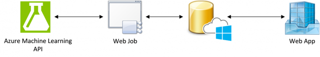
The analysis of new tweets based on “learning” is built using a 4-tier application in Microsoft Azure:

Azure machine learning API:

AzureML provides the prediction model and can be accessed through the web job using the API.

Web job in Azure:

The job (c#) reads new tweets once an hour and passes them to AzureML for classification. The prediction of each tweet is stored in the Azure SQL database.

Azure SQL database:

A dedicated table contains the prediction data of the Tweets.

Web app in Azure:

Serves as a frontend to display Tweets being processed by AzureML

Step-by step

Azure Machine Learning

AzureML is the central component for the forecasts.

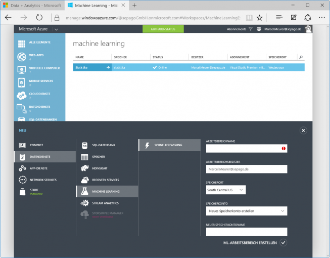
Azure ML Studio can be started in the details pane of the current workspace.

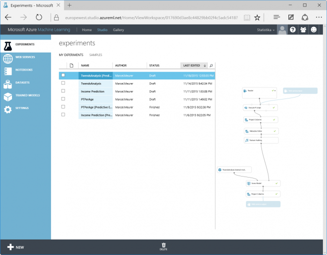
Create the learning experiment

The goals of the training experiment are:

•  Access to the learning data source (our stored Tweets)
•  Data clean up, filtering and assess historical data
•  Format text contained in Tweets and convert it into a machine friendly format
•  Classify Tweets (positive or negative) and train the “machine”
•  Assessment of learning results

Create a new experiment via “new / experiment / blank experiment”. Then give the experiment a user friendly name by changing the grey text into “Experiment created on…”.

Initially the data source of data input and output/reader is included. The source type “Azure SQL Database” allows a direct connection to the database. Required information: server hostname, name of database, user name / password. The following SQL query retrieves the “oldest” 30,000 tweets from the table “Tweets”:

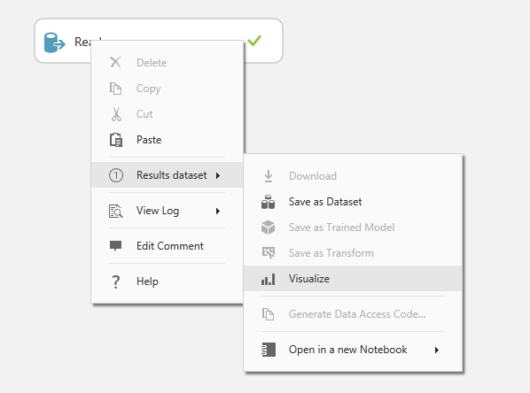
The results of the individual blocks/functions can be displayed via the context menu. This, however, implies that the experiment has been started after configuration. Otherwise the entries under “Result set” are greyed out. The experiment can be started clicking the RUN button at the bottom.

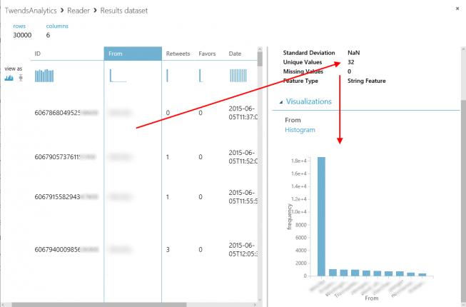
“Result dataset / Visualize” also shows statistical information about the result data set, e.g. the number of different tweeters.

To be able to start the training of the machine we first need a parameter that tells us if a Tweet is qualified as positive or negative. This is done using an R script block. In addition, the R script formats each Tweet for further processing: Any character except A-Z, #: @ and 0-9 will be filtered out. The remaining ones are converted to lowercase (toLower). This reduces complexity , size of data and processing time.

The R script block is being dragged and dropped into the experiment using R Language Modules / Execute R-Script and linked with the data source (the Reader):

The R script utilizes 3 inputs. Here, the input maml.mapInputPort(2) is used:

The first block defines a function that returns “Yes”, if the number of retweets and favors is more than 4 and less than 40. This is the criterion for a positive Tweet in this case now. It’s useful to outsource this code into a function because it is applicable to all records using “sapply”. In “Map Input Port” the input of the R script is assigned to the variable “dataset”. “Separate columns” separates “dataset” into single columns for further processing. “Normalization” formats the Tweet as described above. “IsGood” is the resolution vector of the function to qualify the tweets. “Build dataset” contains the data vectors as a total data stream. This is the result of the script block:

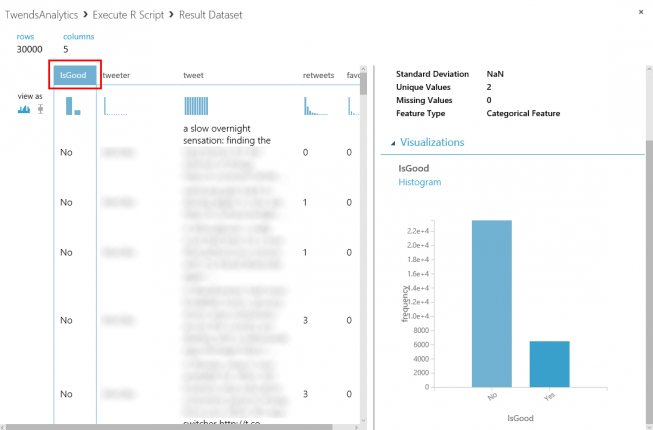
The new column “IsGood” qualifies the Tweets in positive =Yes or No. In this case 22% of the older Tweets are qualified as “positive”.

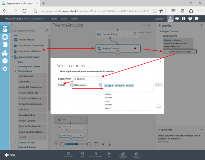
The columns Retweets and Favors are no longer important for the training. Only “IsGood”, “Tweeter” and “Tweet” are required. Using the function “Project Columns in Data Transformation / Manipulation”columns can be explicitly selected/deselected:

In order to evaluate the content of the Tweets it is a good idea to store the formatted text of the Tweets in a hash table. The function “Feature Hashing” located in “Text Analytics” splits data into individual fragments, which are stored in a hash table. In this case the size of the table is 18 bit. This results in a table size of 2 ^ 18 = 262,144 entries. The larger the table, the more accurate the model can be trained. Of course this leads to increased storage costs as well as processing time. During development, this value can be decreased even more to accelerate visualization or troubleshooting. The value N-gramsdefines the size of the fragments that are stored in the hash table and is 2 for 2 characters.

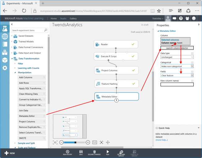
The resulting data stream contains “IsGood”,” Tweeter”, “Tweet” and the hash table. The hash table adds 262,144 columns. For the training the column “Tweet” has become obsolete since the Tweets are replaced by the hash table. ”Tweets” can be marked to be ignored by the training process using “Metadata Editor in Data Transformation / Manipulation”: Select the column “Tweet” and set “Categorical” to “Make non-categorical” as well as “Fields” to “Clear feature”.

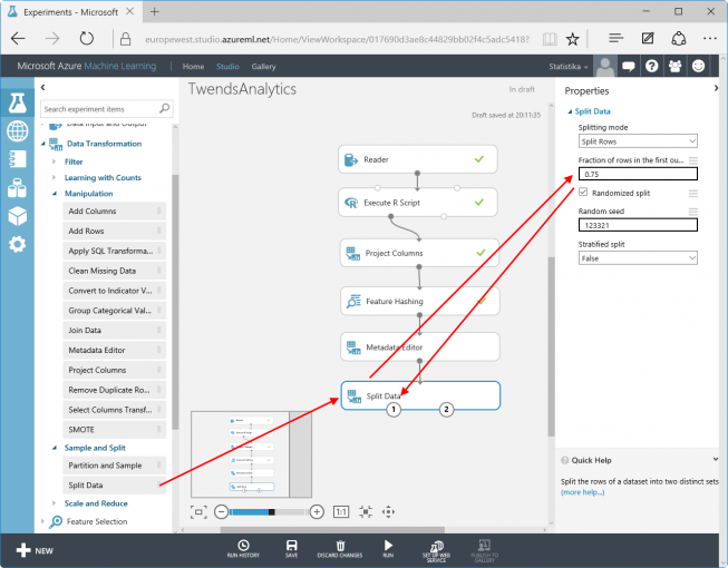
There is one last step, before we can start the actual training: Data has to be split. During the training process one set of data is used to learn with, a second set of data is used to verify the things just learnt. Because the results are known for both parts of the training data (IsGood), the machine is able to evaluate the success of its training. Data Transformation / Sample and Split / Split Data can split data into two sets. Here: 75% to the left output (for training) and the rest to the right output, to check the things just learnt. “Random seed” is an arbitrary value, which initializes the random mechanism.

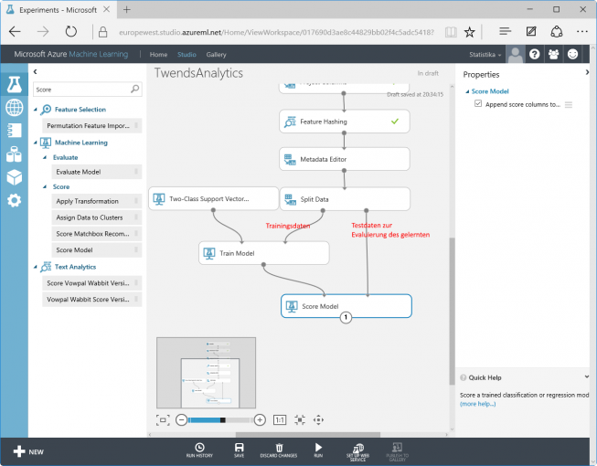
Now, the actual training will be prepared. It consists of a still unskilled Train Model (Machine Learning / Train), the Score Model (“Machine Learning / Score”, used to rate the training) and the selection of the Machine Learning Type (Two-Class Support Vector Machine Learning / Initialize Model / Classification). The choice of the model is based on the challenge the machine has to learn. AzureML offers many different models for different tasks. The one selected here is optimized for processing a high number of columns in the data stream. Simply spoken: The machine learning arranges all the content in a plane and tries to find a path that separates the expected results from the unexpected.

Two of the three modules still have to be configured. For the Two-Class Support Vector Machine the number of iterations is set to 10. To get a better result increase this value (be careful: It also increases processing time). For the Train Model choose the column that contains the result (IsGood) (Note: the column selection may be sluggish due to the high number of columns of the hash table). Connect the data flows:

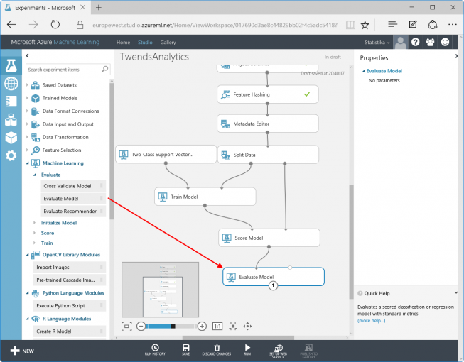
Optionally the Evaluate Model in Machine Learning / Evaluate can be connected. It generates some statistics about the success of the training.

Now the training experiment is complete. A click on RUN starts the training process. The training time depends on the amount of data and processing steps. In this case, it runs a few minutes. Later predictions will be independent of any training processing time: Once learnt, never forgotten (based on a German proverb).

 A right-click on “Evaluate Model / Evaluation Results / Visualize” shows the result of the training and its evaluation. The quality of the model is outlined by the curve “True Positive Rate” over “False Positive Rate”. The more of the 25% test records are located above the diagonal, the better the machine has been trained (and makes better predictions).

This is the difference between a 10-bit and an 18-bit hash table – the 18-bit result shows higher quality:

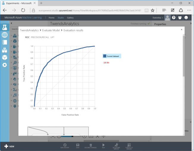
Furthermore, the actual/absolute false predictions are interesting (lower area in the picture).

<- Back   Next ->

14